— Pardon me, do you have the time?
— When do you mean, now or when you asked me? This s*** is moving, Ruth.— George Carlin, Again! (1978)
Getting the time seems easy right? Someone has it, you ask them, and you're done. Well, it's a little more complicated than that.
Let's say you want to set your watch, so you ask the time to a friend. But also imagine voice takes a long, indeterminate amount of time to travel between you and them (alternatively, imagine you want to know what time is it with an extreme precision). When your friend hears your question, it is already too late. They can give you the time it was when they heard the question, but they have no idea when you asked. Now, when you receive their answer you have the same problem. You neither know when they heard your question, nor when they answered. You only know that the time you get corresponds to some point between the moment you asked and the moment you heard the answer.
Now let's say you pick a random point in this interval, and adjust your own watch to that time. Maybe you make an error, but at least you're synchronized with your friend within some tolerance right? No luck! Since it is extremely unlikely both of your watches have exactly the same consistent speed, your watch will drift and wander away from your friend's clock. You could ask again and again. But each time you will get a different error, so your watch will be very noisy (and still drift in between exchanges). Furthermore it seems like a big waste of your... time.
Fortunately for us humans, we don't typically require a high precision compared to the time it takes for sound to travel between two persons speaking to each other. For computers though, it can be crucial to be synchronized within a few microseconds, and network communications can take hundreds of milliseconds. Their clocks are also drifting and jittery, sometimes at an astonishingly high rate. Clearly there have to be ways to mitigate the errors generated by such adverse conditions.
Sources of errors
Before diving into time synchronization protocols, it is useful to clarify what kind of timing errors we're fighting against.
Delay-induced errors
As we already mentioned, one big problem is that there is an uncertainty about when (i.e. how long ago) a measurement happened.
This uncertainty is in most part due to the network latency between hosts, which is not directly measurable. Indeed, the way to measure network latency would be to compare the transmission and reception times of a message between the hosts, but to do that implies that we already have synchronized clocks on both ends...
What can be measured is the round-trip time, i.e. the time a message takes to go from A to B and then back to A. This can obviously be measured with only one clock on A's side. However, keep in mind the round-trip time may not be symmetric, either because the messages didn't take the same route on the outward and return trips, or because network conditions (e.g. congestion) changed during the exchange. Furthermore, the round-trip time changes between each exchange.
We know that the direct travel time from B to A is somewhere between zero and one full round-trip, so if we base our estimate on a symmetric round-trip, our estimation error is bounded by + or - half the roundtrip. The important thing is to remember that the larger the round-trip, the higher the estimation error bound.
Another perhaps less important source of error, is the measurement time of the clock itself. Asking the OS for a clock reading takes some (often variable) time, and the time at which the clock value was read is somewhere between when you asked and when you got the answer.
Clock errors
In addition to network delays, clocks themselves exhibit errors.
- Granularity is the minimal time increment the clock can measure, i.e. the duration between two ticks of the clock. It induces an uncertainty of + or - half that duration.
- Drift is the error caused by a clock oscillator's frequency being slightly off with respect to its specified frequency. This means the clock 'drifts' compared to the "ideal" clock, i.e. it linearly accumulates error over time.
- Wander characterizes the frequency of the oscillator slowly moving (wandering) around its nominal value, e.g. due to temperature changes. It manifests as the low-frequency part of the clock frequency error.
- Jitter is the high-frequency part of the clock frequency error, which can be caused by various sources of noise such as power supply, circuits cross-talk, thermal noise, radiations, etc. It manifests as rapid variations of the duration between each ticks around the average.
Rating your clock
It can be useful to estimate the characteristics of your local clock(s), to choose between different synchronization sources or to evaluate your error intervals. For example NTP implementations use this information to rate clocks and compute accumulated dispersion across several layers of synchronized clocks, as well as to adapt the time constants in their mitigation algorithm.
You can measure your clock granularity by repeatedly (e.g. a few thousand times) taking close clock measurements in a loop and keeping the minimum increment.
You can get an estimate of the average read time by timing a loop where you repeatedly ask clock measurement and divide by the number of iterations.
Estimating the other sources of error actually requires comparing your clock to another (hopefully more accurate) source. NTP estimates these characteristics as part of its mitigation algorithms, as we detail below.
The Network Time Protocol
The ubiquitous solution to time synchronization on computer networks is the Network Time Protocol. It allows to synchronize clocks to a common reference (usually Coordinated Universal Time) with an accuracy of a few milliseconds over the Internet, and can typically provide sub-millisecond accuracy on local networks. NTP was pioneered by Pr. David Mills, whose webpage is a treasure trove of information about time synchronization. The protocol was described in various RFCs, from its first version (RFC1059) to the current fourth RFC5905.
Other clock synchronization protocols exist, e.g. PTP (IEEE 1588-2019), and some implementations of NTP such as Chrony include different error mitigation techniques than those described by the specification.
I will focus here on NTP since it's the most documented and widely used, and it doesn't require specialized hardware like PTP.
The NTP network
To maintain a consistent notion of time across the internet, you first need some reference time signal, which is typically provided by atomic clocks. Since it is neither practical nor desirable to connect every computer in the world to these atomic clocks, the time signal is distributed across a network of peers organized in several strata. Primary servers sit at stratum 1 and are directly connected (through wire or radio) to a reference clock. Peers at stratum 2 can synchronize on servers at stratum 1 or 2, and act as synchronization sources for peers at stratum 3. The layering continues up to stratum 15. Stratum 16 represents unsynchronized devices.
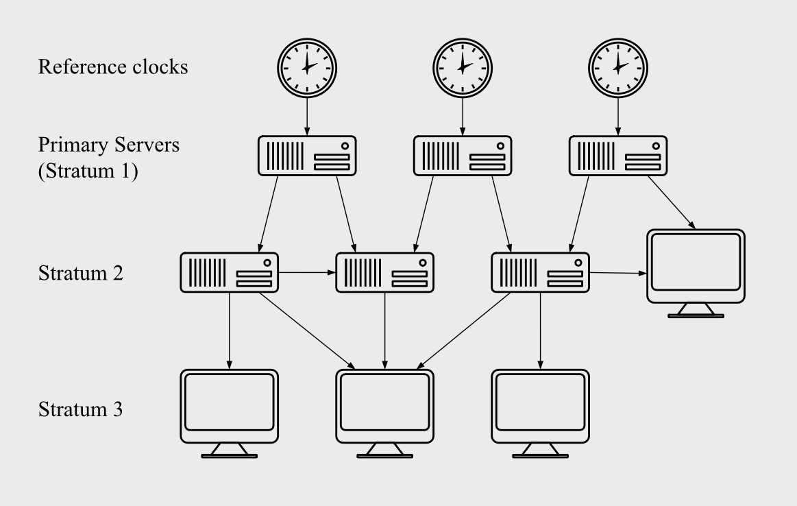
A flow graph of the NTP hierarchy. (vector version)
The protocol selects sources in order to avoid loops and minimize the round-trip delay to a primary server. As such, peers collaborate to automatically reorganize the network to produce the most accurate time, even in the presence of failures in the network.
NTP time formats
NTP doesn't really care about human calendar dates or time zones. It only needs to unambiguously represent instants in time, and be able to compute durations between instants. NTP uses two different formats to represent points in time:
- NTP timestamp
- Fractional seconds since January 1, 1900 UTC (even if UTC didn't exist back then, see above).
- Uses 64 bit fixed point format. The 32 most significant bits denote the number of seconds, the 32 least significant bits denote fractional seconds. The smallest time increment is thus $2^{-32}$ seconds (232 picoseconds). The maximum representable time range is approximately 136 years.
- NTP date
- Uses 128 bits as follows: a 32-bit signed era number, and a 96-bit fixed point era offset (32 bits for seconds and 64 bits for fractional seconds).
- Covers the whole universe's existence with a precision well below any duration that can be directly measured.
NTP architecture
Now let's see the implementation of one node of the network. The following diagram shows the various stages of the pipeline used to collect time information and mitigate errors caused by network delays and clock inaccuracies. I'll explain each one in a short paragraph and give links to the relevant parts of the RFC, and to other references if you want to dig deeper.
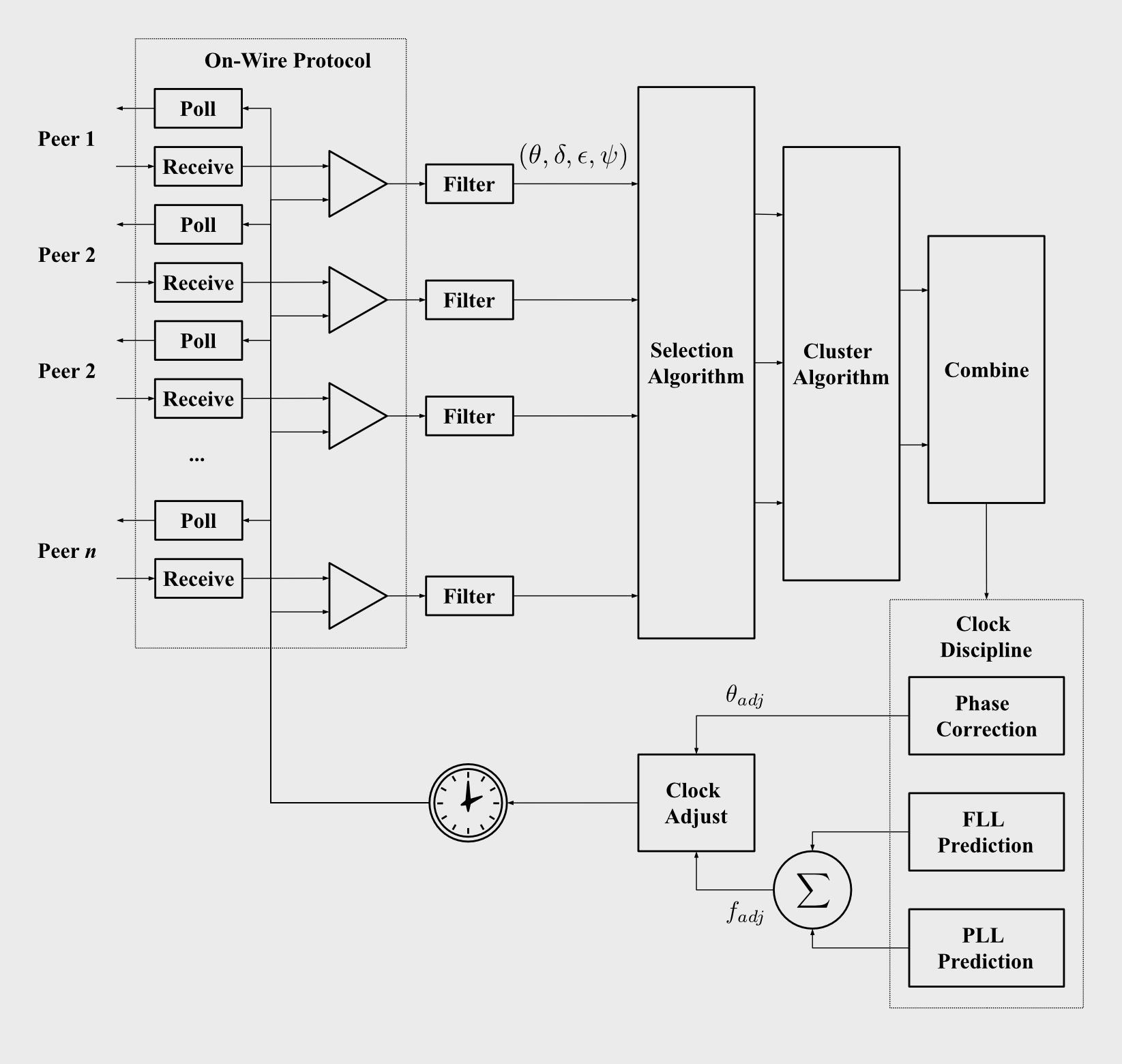
An overview of the NTP architecture. (vector version)
On-wire protocol
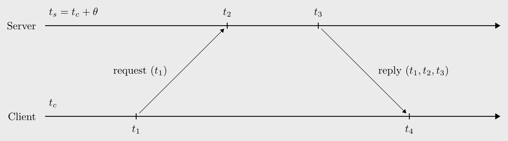
The first stage consists of getting time estimates from each peer. In the simplest mode of operations, the node polls a peer by sending a request packet timestamped with the transmission time, $t_1$. Upon reception of the request, the peer stores a timestamp $t_2$, processes the message, and sends a response packet containing $t_1$, $t_2$ and the response transmission time $t_3$. The node receives the response at time $t_4$.
The node then computes the tuple $(\delta, \theta, \epsilon)$, where:
- $\delta$ is the round-trip delay.
- $\theta$ is the estimated offset of the server clock with respect to the local clock.
- $\varepsilon$ is the dispersion of the sample, i.e. the maximum error due to the frequency tolerances $\varphi_p$ and $\varphi_c$ of the peer's clock and of the client's clock, and the time elapsed since the request was sent.
$\begin{align*} \delta = (t_4 - t_1) - (t_3 - t_2),\qquad \theta = ((t_2 - t_1) + (t_3 - t_4))/2,\qquad \varepsilon = \varphi_p \times \varphi_c \times \delta \end{align*}$
Note that peers also transmit the delay and dispersion statistics accumulated at each stratum from the root down to the peer, yielding the root delay and dispersion, $\theta_r$ and $\varepsilon_r$. These statistics are used to assess the "quality" of the samples computed from each peer.
Simple NTP clients that are only synchronized to one server, that don't act as a source for other peers, and that don't need a high precision, can implement only the on-wire protocol and directly use $\theta$ to correct their local clock. However this estimate is vulnerable to network jitter, delay asymmetry, clock drift and wander. To get better precision, the samples produced by the on-wire protocol must be processed by a number of mitigation algorithms.
Links: Mills, Analysis and Simulation of the NTP On-Wire Protocols, RFC5905 - section 8, SNTP (RFC4330)
Clock filter
The clock filter is a shift register containing the last 8 samples produced by the on-wire protocol. The filter algorithm selects the sample with maximum expected accuracy. It is based on the observations that:
- The samples with the lowest network delay were likely to exhibit a low error at the time they were produced.
- Older samples carry more accuracy than newer ones due to clock drift.
As a new sample is pushed to the register, it evicts the oldest sample. The dispersion values of the other samples are then incremented by $\varphi_c\times\Delta_t$, where $\Delta_t$ is the time elapsed since the last update from the server. A distance metric $\lambda_i$ is associated to each sample:
$\lambda_i = \frac{\delta_i}{2}+\varepsilon_i ,.$
The samples are then sorted in a temporary list by increasing value of $\lambda_i$. The list is pruned to leave only samples whose dispersion is less than a given maximum. The first sample in the list is chosen as the new best candidate, likely to give the most accurate estimate of the time offset $\theta$. However it is only used if it is not older than the last selected sample.
The peer's dispersion $\varepsilon_p$ is computed as an exponentially weighted average of the sorted samples' dispersions:
$\varepsilon_p = \sum_{i=0}^{N-1}\frac{\varepsilon_i}{2^{(i+1)}} ,.$
The server's jitter $\psi_p$ is computed as the root mean square (RMS) of the offsets differences with respect to the offset of the first sample's in the list [NOTE(hayden): This sentence is difficult to read -- it may be because of the multiple forms of gramatical possessiveness. There also might be some typos in that regard][NOTE(martin): let me know if this one works better: The server's jitter $\psi_p$ is computed as the root mean square (RMS) of the differences of each offset with the first offset in the list]:
$\psi_p = \frac{1}{n-1}\sqrt{\sum_{i=0}^{N-1}(\theta_0-\theta_i)^2} ,.$
Links: Mills, Clock Filter Algorithm, RFC5905 - section 10
Clock selection
The estimates we get from the clock filters of each peer can be in contradiction, either because of network perturbation or because some peers are faulty (or malicious!). The clock selection algorithm tries find a majority group of peers with consistent time estimates (the "truechimers"), and eliminates the other peers (the "falsetickers").
The algorithm is based on the observation that for a non-faulty peer, the time offset error at the time of measurement is bounded by half the round-trip delay to the reference clock. This bound then increases with the age of the sample, due to the accumulated dispersion.
The true offset thus lies in the correctness interval $[\theta - \lambda_r, \theta + \lambda_r]$ ($\lambda_r$ being the accumulated distance to the root). Two peers whose correctness intervals do not intersect can not possibly agree on the time, and one of them must be wrong. The algorithm tries to find the biggest majority of candidates whose correctness intervals share a common intersection, and discards the other candidates.
Links: Mills, Clock Select Algorithm, RFC5905 - section 11.2.1, Marzullo and Owicki, 1983
Cluster algorithm
Once falsetickers have been eliminated, truechimers are placed in a survivor list, that is pruned by the cluster algorithm in a series of rounds.
For each candidate, it computes the selection jitter, which is the root mean square of offset differences between this candidate and all other peers. Candidates are ranked by their selection jitter and the candidate with the greatest one is pruned from the survivor list.
The cluster algorithm continues until a specified minimum of survivors remain, or until the maximum selection jitter is less than the minimum peer jitter (in which case removing the outlier wouldn't improve the accuracy of the selection).
To get some grasp of why it is designed that way, imagine all samples are coming from the same "idealized" peer, and that we select one "most likely accurate" sample. Then, as we already saw in the clock filter algorithm, we can compute the jitter of that idealized peer. The selection jitter is essentially a measure of the jitter implied by the decision to consider that sample the most accurate. Now to understand the termination condition, remember that each sample is produced by a peer that itself exhibits some jitter. There is no point in trying to get a better jitter from the combination of all samples, than the minimum peer jitter.
Links: Mills, Cluster Algorithm, RFC5905 - section 11.2.2
Combine
The combined offset and jitter are computed as an average of the survivor's offsets and jitters, weighted by the inverse of the root server's distance.
Clock discipline
The combined estimates are passed to the clock discipline algorithm which implements a feedback control loop, whose role is to direct the local system clock towards the reference clock. At its core the clock discipline consists of the non linear combination of a phase locked loop (PLL) and a frequency locked loop (FLL). It results in a frequency correction and a phase correction.
The discipline is further enhanced by a state machine that is designed to adapt the polling interval, and the relative contribution of the PLL and FLL, in order to allow fast initial convergence and high stability in steady state. It also handles special situations such as bursts of high latency and jitter caused by temporarily degraded network conditions.
Links: Mills, Clock Discipline Algorithm, Mills, Clock State Machine, Mills, Clock Displine Principles, RFC5905 - section 11.3
Clock adjust
The clock adjust process is called every second to adjust the system clock. It sums the frequency correction and a percentage of the offset correction to produce an adjustment value. The residual offset correction then replaces the offset correction. Thus, the offset correction decays exponentially over time. When the time since the last poll exceeds the poll interval, the clock adjust process triggers a new poll.
It is worth noting that because it is crucially important to preserve a monotony property, the system clock is never actually stepped back or forth: instead, the system usually throttles the clock up or down until the desired correction has been achieved.
Links: RFC5905 - section 12
And this concludes our tour of NTP!
Written by Martin Fouilleul.